Fundamentals of FEA

Finite Element Analysis (FEA), also known as the Finite Element Method (FEM), is a numerical technique for describing physical phenomena in terms of partial differential equations. Finite element analysis is widely used in many engineering disciplines for solving structural mechanics, vibration, heat transfer, electromagnetics, and other problems.

You can use the FEM to predict the behavior of mechanical, thermal, and electrical systems under their operating conditions, to reduce the design cycle time, and to improve overall system performance.

FEA model is composed of several different components that together describe the physical problem to be analyzed and the results to be obtained. The basic steps in any FEA process are as follows:

Geometric Representation

Creates the geometric features of the system to be analyzed and stored in a CAD database.

Discretization of Geometry

Splits the geometry into relatively small and simple geometric entities, called finite elements. This discretization process is better known as meshing. The elements are called “finite” to emphasize the fact that they are not infinitesimally small, but only reasonably small in comparison to the overall model size.

Finite elements and nodes define the basic geometry of the physical structure being modeled.

Each element in the model represents a discrete portion of the physical structure, which is, in turn, represented by many interconnected elements. Elements are connected to one another by shared nodes. The coordinates of the nodes and the connectivity of the elements—that is, which nodes belong to which elements—comprise the model geometry. The collection of all the elements and nodes in a model is called the mesh. Generally, the mesh is only an approximation of the actual geometry of the structure.

The element type and the overall number of elements used in the mesh affect the results obtained from a simulation. The greater the mesh density (that is, the greater the number of elements in the mesh), the more accurate the results. As the mesh density increases, the analysis results converge to a unique solution, and the computer time required for the analysis increases. The solution obtained from the numerical model is generally an approximation to the solution of the physical problem being simulated. The extent of the approximations made in the model's geometry, material behavior, boundary conditions, and loading determines how well the numerical simulation matches the physical problem.

Element Characterization

Develops the equations that describe the behavior of each element. Material properties for each element are considered in the formulation of the governing equations. This involves choosing a displacement function within each element. Linear and quadratic polynomials are frequently used functions.

Element section properties

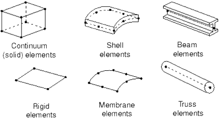
The choice of the appropriate element is very important for the simulation of the physical problem. Element libraries include a wide range of elements that are simple geometric shapes with one, two, or three dimensions.

For example, in case of structural analysis, continuum or solid elements are appropriate for bulky or complex 3D models. Shell elements are suitable for thin parts with thickness significantly smaller than the other dimensions. Beam elements are suitable for structural members where the length is significantly greater than the other two dimensions.

Common element families

Material Data

Material properties for all elements must be specified. While high-quality material data are often difficult to obtain, particularly for the more complex material models, the validity of the simulation results is limited by the availability of accurate material data.

Analysis Type

Depending on the type of applied load environment, the inclusion of inertia effects, and material properties, the appropriate analysis type must be selected for the simulation. Common analysis types include linear static, nonlinear static, dynamic, buckling, heat transfer, fatigue, and optimization.

In a static analysis, the long-term response of the structure to the applied loads (which are applied gradually and slowly until they reach their full magnitude) is obtained. In cases where the loads are changing with time or frequency, a dynamic analysis is required. For example, you perform dynamic analysis to simulate the effect of an impact load on a component or the response of a building during an earthquake.

A nonlinear structural problem is one in which the structure's stiffness changes as it deforms. All physical structures exhibit nonlinear behavior. Linear analysis is a convenient approximation that is often adequate for design purposes. It is obviously inadequate for many structural simulations including manufacturing processes, such as forging or stamping, crash analyses, and analyses of rubber components, such as tires or engine mounts.

Loads and Boundary Conditions

The application of loads distorts the physical structure and thus creates stress in it. Boundary conditions are used to constrain portions of the model to remain fixed (zero displacements) or to move by a prescribed amount (nonzero displacements).

The most common forms of loading include:

• Point loads
• Pressure loads on surfaces
• Distributed tractions on surfaces
• Distributed edge loads and moments on shell edges
• Body forces, such as the force of gravity
• Thermal loads

In a static stress analysis, adequate boundary conditions must be used to prevent the model from moving as a rigid body in any direction; otherwise, unrestrained rigid body motion causes the simulation to stop prematurely. The potential rigid body motions depend on the dimensionality of the model.

Solution of Equations

Provides the solution for the unknown nodal degrees of freedom (or generalized displacements).

Postprocessing

Obtains visualization plots for quantities of interest, such as stresses and strains.

👉 Please check the below video to understand how to perform the above steps in the 3DEXPERIENCE Platform.