Introduction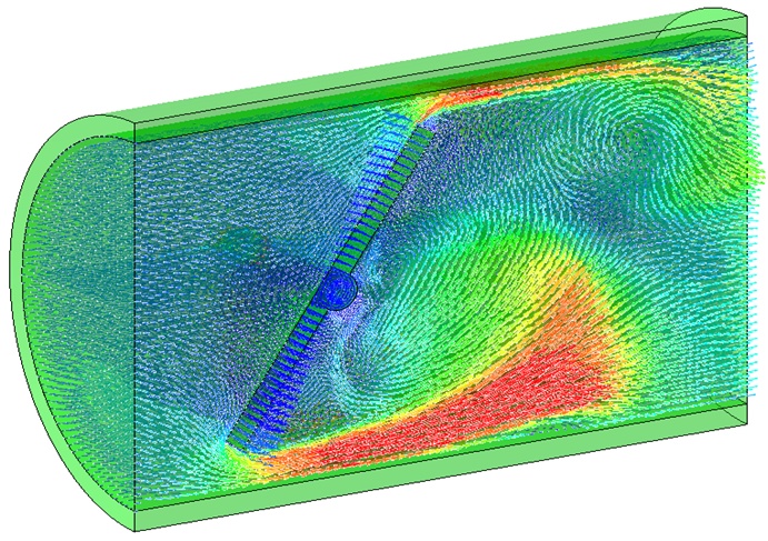

We demonstrate setting up an FSI simulation using the example of a butterfly valve subject to rigid body rotation. The various steps to be followed while setting up an FSI analysis is as follows:

• Develop the CFD model (Abaqus/CFD)
  • Define the fluid-structure interface wall boundary
    • Co-locate the interface boundary between the fluid and the structural domains
• Verify your CFD-only analysis by prescribing velocities or temperatures at the interface wall
  • For FSI, prescribe mesh displacements to exercise ALE 

• Develop the structural model (Abaqus/Standard or Abaqus/Explicit)
  • Identify the fluid-structure interfaces
    • Co-locate the interface boundary between the fluid and the structural domains
• Verify the “dry” structural model using “assumed” pressure/heat flux loads at the interface
  • Apply pressure/heat flux load magnitudes that are reasonable and similar to the expected fluid loads 

• Interconnect the structural and CFD models for the co-simulation
  • Delete the “assumed loads”
  • Define the fluid-structure interaction and the exchange variables on a co-simulation region
    • The co-simulation region defines boundary conditions for both the structural and the CFD model 

• Run the FSI analysis
  • Create co-execution jobs 

• Postprocess the structural and CFD solution

  Fluid model

The half-symmatry Abaqus/CFD model representing the fluid domain is shown in Figure 1.  The length of the valve itself is 0.042m.  The computational model dimensions have been chosen to mimic the pipe that the valve operates in. The diameter of the pipe is 0.045m and the length is 0.075m. The model consists of 532379 tetrahedral fluid elements (FC3D4). The simulation is run for a total simulation time of 0.3 s. The CFD model includes a surface definition representing the region of the fluid which interacts with the cylinder surface.  It will be used to define the co-simulation interaction with the Abaqus/Standard model. 

Figure 1. CFD model

Material Properties

The fluid is modeled as an incompressible Newtonian fluid.  The properties of the fluid are chosen to achieve a flow Reynolds number of 4200 based on valves’s diameter and the inlet velocity.  The fluid density is chosen to be 1000 kg/m3 and viscosity is 0.001 Pa∙sec.

Flow Solver

The Abaqus/CFD procedure invokes a transient incompressible turbulent flow analysis.  Automatic time incrementation based on a fixed Courant-Freidrichs-Lewy (CFL) condition is used. The Spalart-Allmaras turbulence model is chosen to simulate turbulence.

The following ‘flow’ boundary conditions are applied to the fluid. 

1. Inlet:  An inlet velocity of 0.1 m/sec is applied
2. Outlet:  An outlet boundary condition is specified with the fluid pressure set to zero. 
3. Pipe Wall:  A no-slip/no-penetration wall boundary condition is applied at the pipe wall. All velocity components are set equal to zero.   
4. Symmetry:  The velocity normal to the symmetry planes (Vy) is assumed to be zero to constrain the out-of-plane flow.

The following ‘mesh’ boundary conditions are applied to the fluid. 

1. Inlet:  Define a ‘Mechanical’ category boundary condition of type ‘Displacement/Rotation’ and constrain mesh motion in the U3 direction by setting U3=0.
2. Outlet:  Constrain mesh motion in the U3 direction by setting U3=0.
3. Pipe Wall:  Constrain all 3 components of mesh motion to zero: U1=U2=U3=0
4. Symmetry:  Constrain mesh motion in the U2 direction by setting U2=0.

Initial Conditions

The following predefined fi.elds are supplies to start the simulation: Initial kinematic eddy viscosity of 3.0E-6

Define the FSI interaction

Create an interaction of type Fluid-Structure Co-simulation boundary and choose the valve surface as the surface to which the interaction will be applied. 

Structure Model

The Abaqus/Standard model of the pipe-valve assembly is shown in Figure 1.

Figure 2 Structural model for Pipe-Valve assembly

The structural model in Abaqus/Standard is comprised of first-order hexahedral stress/displacement elements (C3D8R).  A total of 35000 elements are used to define the assembly.  The valve’s surface interacts with the surrounding fluid and hence it is used to define the co-simulation interaction with the Abaqus/CFD model.  

Material Properties

A density of 7800 kg/m3, Young’s modulus of 200 GPa, and Poisson’s ratio of 0.3 are used to define the cylinder’s material properties.    

Constraints

A rigid-body constraint has been applied to the pipe to model the pipe as a rigid body. A coupling constraint is applied to the valve to rotate the valve as a rigid body based on a reference point

Structure Solver

The Abaqus/Standard procedure invokes an implicit dynamic analysis step. An initial time increment of 0.0001 s is used; however, the time increment can change depending on whether the structural or CFD model is dictating the time increment size.  The built-in time incrementation strategy is used where the co-simulation coupling time is chosen as the minimum of the time increments dictated by the structural and CFD models.  The total simulation time is chosen to be 0.3 s

Boundary Conditions

The following boundary conditions are applied to the structure assembly

1. Pipe: Constrain all degrees of freedom of the pipe referent point
2. Valve: Apply an angular velocity component to the valve reference point in the y-direction of UR2=-0.0873 and constrain all other degrees of freedom.
3. Create an interaction of type Fluid-Structure Co-simulation boundary and choose the valve surface as the surface to which the interaction will be applied

Define the FSI interaction

Creating a co-execution analysis

In order to perform the fluid-structure interaction analysis, the Abaqus/Standard and Abaqus/CFD jobs need to execute together.  A co-simulation is performed where the two solvers exchange information at each co-simulation target time.  The co-simulation target time is automatically chosen as the minimum of the time increments required by the structural and CFD solvers.  In order to facilitate the co-simulation of the two analyses, the co-execution job procedure is used.  A co-execution job creates two analysis jobs and runs them simultaneously.  It also automatically provides the driver options needed for communication between the two analysis jobs.   

Running the co-simulation analysis

Launch the co-execution job from within Abaqus/CAE. 

1. Click mouse button 3 on the co-execution job. 
2. From the menu that appears, select Submit. 

This launches the co-execution job.  Both the Abaqus/Standard and Abaqus/CFD jobs will be launched.  

Monitoring the co-execution analysis

While the co-execution is running, you can monitor its progress. 

1. Click mouse-button 3 on the CFD analysis job name and select Monitor from the menu that appears. 
2. The job monitor appears.  Note that time incrementation information, divergence (RMS) and kinetic energy is updated every time increment.

Viewing the results

Once the co-execution completes, do the following: 

1. Click mouse button 3 on the co-execution.
2. From the menu that appears, select Results.

The output database files for both the fluid and structure jobs are opened simultaneously in the Visualization module and are overlaid in the viewport. 

1. Toggle off the overlay plot option  in the toolbox.
2. Create pressure and velocity contour plots
3. Create velocity contour plots and animate them. A plot of the velocity contour is shown below

Figure 3. Velocity vectors across the valve.

Video Demo

A detailed video of setting up the simulation from scratch and visualizing the results is attached herewith.

The CAE file is also attached here.